Modeling the spread of COVID-19 in UCLA classrooms
What would happen if UCLA students returned in the fall to take in-person classes? We explore the potential spread of COVID-19 among students on UCLA’s campus.
By
Radhika Ahuja,
Charlotte Huang,
Sydney Kovach,
Laurel Woods
May 12, 2020
Key Takeaways
According to our model of the undergraduate student network, each UCLA student shares a class with 228 other students on average.
Our simulation shows that with an R0 value of 5.7, 94% of UCLA undergraduates could be infected by the end of fall quarter, and with an R0 value of 2.0, 8% of UCLA undergraduates could be infected.
In the middle of a global pandemic, uncertainty has become the new normal. Many states across the country are now beginning to lift restrictions, but colleges must weigh the difficult decision of how to keep students and staff safe while still providing a quality education. While UCLA has already decided to move summer sessions A and C online, the fate of fall quarter is still up in the air. Crowded lecture halls and dorm rooms make it nearly impossible for students to practice social distancing without a disruption to normal college life. As UCLA grapples with whether to welcome students back to campus in the fall, The Stack examines how quickly COVID-19 could spread through the undergraduate student body. Inspired by professor Kim Weeden’s model of course enrollment networks at Cornell University, we created our own model of how connected UCLA students are based on the classes they enroll in. We also thank Professor Mason Porter and Professor Stephanie Wang from the UCLA Math department for providing guidance on modeling the student networks and for their constructive comments in the development of this piece.
Methods and Assumptions
Our model looks solely at the spread of COVID-19 through classes and does not take into account interactions students may have through dorm rooms, dining halls, campus organizations or other social aspects of student life. We assume that any student who shares a class with an infected student is exposed to the virus and could become infected. Additionally, the model only takes undergraduate students into consideration. In particular, a realistic picture of the campus includes many more affected groups, like graduate students, faculty, administrative staff, on-campus and dining workers, many of whom are more likely to be in a higher risk category than undergraduate students. However, to keep the model simple and its implementation feasible given the available data, we only factor in undergraduate students. It should also be noted that, although the studies referenced in this article have not yet been peer-reviewed, this is common for coronavirus-related studies because of their newness.
The incubation period for COVID-19 is typically five to six days, though it can take anywhere between one to 14 days to develop symptoms after exposure, if symptoms do develop. LA County offers free COVID-19 testing to all residents, including three testing sites within five miles of UCLA, but same-day and next-day appointments are prioritized for front-line workers and symptomatic patients. We assume that UCLA students will get tested seven days after exposure on average.
Ideally, once someone tests positive, they will self-isolate either the same day or the next day; therefore, we assume that infected students that become symptomatic will be contagious and spread COVID-19 for about a week. However, asymptomatic spread is also significant; according to an NPR interview with Robert Redfield, director of the Centers for Disease Control and Prevention, up to 25% of people with COVID-19 may never show symptoms and are therefore less likely to seek testing and self-isolate. Moreover, a study stated that 40% to 80% of transmissions could occur from individuals who have not shown symptoms.
R0, pronounced “R-naught” and referred to as the “basic reproduction number,” measures how many others an infected individual will infect. An R0 below one means that the virus will die out over time whereas an R0 above one means there will be exponential growth, as has been seen in the United States. The value of R0 can vary across regions as it depends on population density and the amount of human contact, so the more social interactions that take place, the higher R0 will be. In California, social distancing and shelter-at-home orders have helped to reduce R0 below the nation-wide levels and to flatten the curve of new infections. However, if in-person classes take place in the fall, the infection rate at UCLA would be higher than the current R0 in a locked-down Los Angeles. For our model, we allow the user to explore the spread based on different R0 values. An R0 of 5.7 was found to be the median R0 value calculated by a study posted on the CDC website based on data from China. Other studies cite much smaller R0 values. The New York Times estimated that the pathogen that causes COVID-19 has an R0 value ranging from 2.0 to 2.5, a study from the WHO also cites an R0 of 2.0 to 2.5. Because of the multitude of studies on R0, our model shows the effects of an R0 ranging from 0.0 to 5.7.
We started with a single infected student at UCLA. An infected student will infect an average of R0 of their classmates over the period of one week. Each classmate has a certain probability of being infected based on the R0 and the number of classmates the original infected student has. Although research is still being done on immunity to COVID-19, we assumed that once a student has recovered, they will not be infected again.
Modeling the Student Network
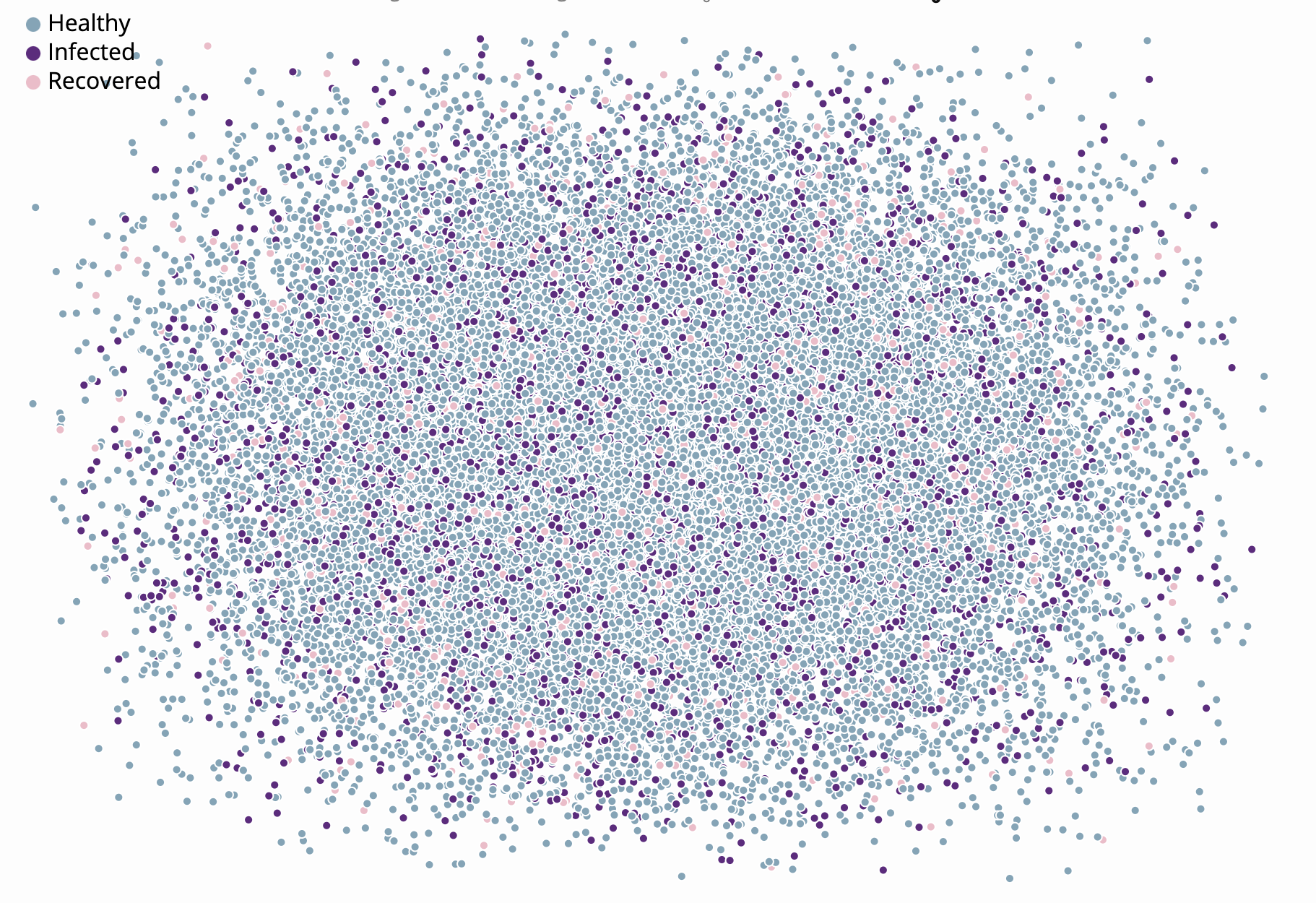
The graph below models a typical quarter at UCLA, with each node representing an undergraduate student. Using fall 2019 data provided by the Office of Academic Planning and Budget of how many students are in each major, each student was placed in one of 76 departments and randomly assigned to three courses that were either within their department or were GEs, using a stochastic block model. Each student is then assumed to be connected to every other student they share a class with, and the virus can be transmitted between connected students.
Interdepartmental connectivity in this model arises primarily from degree/school-level requirements like general education, diversity and language. Some other cases like interdepartmental requirements and cross-listing for individual majors, minors, and double majors are not taken into account. In general, these factors are likely to make the model more interconnected and as such our version is a more conservative picture. Some other niche cases like students coming in with transfer credit or students who waive out of certain requirements using diagnostic tests are not considered, i.e., it is assumed that every student takes all their required courses at UCLA.
To explore the visualization, drag the time slider forward through the weeks of fall 2020 or press play to automate it. Each week, an infected student will infect an average of R0 students. The value of R0, set to zero by default, can also be adjusted with the slider above the graph to explore different rates of infection.
UCLA could maintain a small R0 if the university implements mandatory social distancing in classrooms, requires the wearing of masks or provides ample sanitizing products to all classrooms and lecture halls. Any combination of these measures would decrease the spread of the virus.
Student Network
Drag the slider to change the value of R0
R0 = 0.0
week of fall quarter
In our model network, students had an average of 228 connections. We ran the simulation 100 times from week 0 to finals week with an R0 value of 5.7, and found that on average, 94% of students were infected by the end of fall quarter. The peak of new cases occurred at week 6 with over 11,000 new cases. With a smaller R0 of 2.0, we found that 8% of students were infected by the end of fall quarter.
We also calculated the average number of infections over 100 runs for several different values of R0. The following chart shows the number of people infected on average through the 11 weeks, for varying values of R0:
The potential spread of the virus depicted above does not take into account interactions in shared spaces such as Bruin Walk, libraries, dining halls, etc. or the fact that the same lecture hall is used, i.e., the same chairs are reused and such surfaces might be a source of infection. These models also do not show the potential spread through shared living spaces such as dorms and apartments. Consequently, COVID-19 could be much more infectious through the UCLA community than the models above show. In fear of outbreaks, California State University campuses will remain closed for the Fall 2020 semester, and the 23 universities in this system will proceed with primarily virtual instruction. UCLA has yet to make a decision on whether the Fall 2020 quarter will be held virtually or whether there will be some in-person instruction.
As of May 11, there are over 1.3 million confirmed cases and over 80,000 deaths in the U.S. In LA County, there are over 32,00 confirmed cases and over 1,500 deaths. LA County is offering free coronavirus tests for all residents and working to test up to 10,000 people every day, with each site capable of running 100 to 500 tests per day. Up to one in four COVID-19 patients may remain asymptomatic and never quarantine. Asymptomatic carriers may therefore be more likely to spread the virus than those who show symptoms, get tested and quarantine themselves. It is crucial to practice social distancing, wash hands and wear a cloth mask to prevent the virus from spreading, according to the CDC.
UCLA is a large school with a very well-connected student network posing numerous challenges for reopening the university in Fall.
For more updates on coronavirus news relevant to UCLA, visit the Daily Bruin’s coronavirus dashboard. For more information about how students have been affected by the pandemic, visit the Daily Bruin’s “Unfinished Stories” project. To schedule a free COVID-19 test in LA County or learn more about testing, click here. More information about the coronavirus and COVID-19 from UCLA Health can be found here.
More on Stochastic Block Models
A stochastic block model considers a set of student communities, grouped by department, such as mathematics, art history or psychology. So for example, consider a three-department school: Sciences with 200 students, Business with 150 students and Humanities with 170 students. The student communities set is then [200, 150, 170].
Then a matrix A defines the probabilities used to randomly assign students from each department to courses in other departments. Celli, j of A represents the probability that a student housed in department i will take a course in department j. For this example, there’s a probability of 0.7 that a sciences student will take a sciences class, a 0.1 probability they will take a business class, and a 0.2 probability they will take a humanities class.
This example has simulated probabilities, but the real probabilities in our model are based on the number of GE, diversity and language courses in each major. So if a College of Letters and Science student in the mathematics department takes 140 units of major courses and 40 units of GEs, then the probability of the student being enrolled in the mathematics department is \(\frac{140}{180}\), and, in the other GE-offering departments, is \(\frac{40}{180}\), which in turn are distributed by department. So if there are three GE courses offered in total, with two of them being offered in department A and one being offered in department B, department A will have probability \(\frac{2}{3} * \frac{40}{180}\), and department B will have probability \(\frac{1}{3} * \frac{40}{180}\).
$$
This example has simulated probabilities, but the real probabilities in our model are based on the number of GE, diversity and language courses in each major. So if a College of Letters and Science student in the mathematics department takes 140 units of major courses and 40 units of GEs, then the probability of the student being enrolled in the mathematics department is \(\frac{140}{180}\), and, in the other GE-offering departments, is \(\frac{40}{180}\), which in turn are distributed by department. So if there are three GE courses offered in total, with two of them being offered in department A and one being offered in department B, department A will have probability \(\frac{2}{3} * \frac{40}{180}\), and department B will have probability \(\frac{1}{3} * \frac{40}{180}\).
To learn more about how this article was made, watch the video below:
AUTHORS
Radhika Ahuja
Stack Developer
Radhika was a math of computation student. Outside of school, she enjoys writing, dance, cooking and other things creative.
Charlotte Huang
Stack Developer
Charlotte was an applied math and cognitive science student. Outside of math and data, she enjoys reading, watching K-Drama and listening to K-Pop.
Sydney Kovach
Stack Developer
Sydney Kovach was a global Studies and geography student who loves dancing and taking yoga classes in her free time.
Laurel Woods
2021-22 Data Editor
Laurel was a cognitive science and digital humanities student. She was the 2021-22 Data Editor. She loves anything outdoorsy, especially if her dog is there.